Political Twitter Part 3

Exploratory Data Analysis

---

Exploratory Data Analysis (EDA) is different when being performed on text data. Analysis performed on text works with representations of the data rather than the original data itself. Here we will perform EDA using the cleaned text from Part 2.

Click Here for full code notebook

Check for Data Imbalance

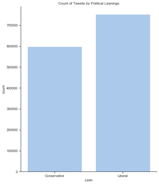
I have close to equal proportions of liberal and conservative tweets. 2020 is an election year and the Democrats have a large field of hopefuls so it is no surprise that they have slightly more tweets.

# read in df from pickle file
tweets_clean_df = pd.read_pickle('outdata/tweets_clean_df.pkl')

# get counts by political group
counts = tweets_clean_df.groupby("class").agg(
    count=('class',"count")).reset_index()

# Generate full text lables for use in graph
counts["Lean"] = np.where(counts['class']=='L',"Liberal", "Conservative")

# prepare data for plotting
counts = counts[["Lean", "count"]]

# begin plot
sns.set(style="ticks")

# Initialize the matplotlib figure
f, ax1 = plt.subplots(figsize=(8,10))

# Barplot of parties
sns.set_color_codes("pastel")
g = sns.barplot(x="Lean",
            y="count",
            data=counts,
            label="Total",
            color="b",
            ax=ax1).set_title("Count of Tweets by Political Leanings")

sns.despine()

# separate corpus into Liberal and and Conservative lists for analysis
lib_tweets = tweets_clean_df[tweets_clean_df['class']=='L']['clean_tweets'].tolist()
con_tweets = tweets_clean_df[tweets_clean_df['class']=='C']['clean_tweets'].tolist()

Use N-Gram counts to discover top themes

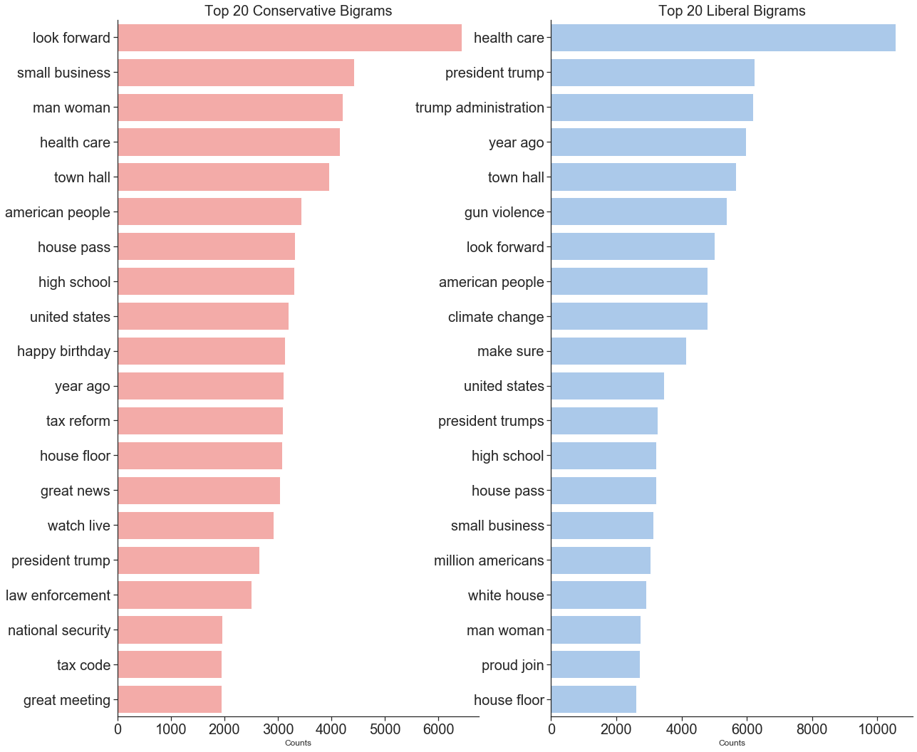
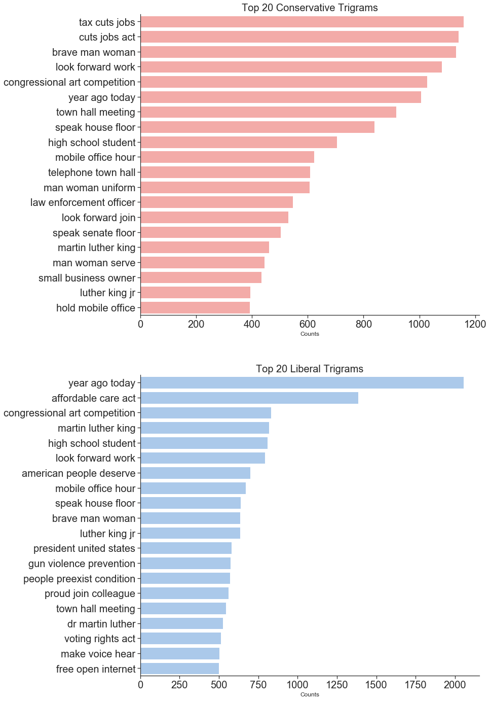
A common Natural Language Processing technique for identifying themes in a text is to count the occurrences of n-grams. N-grams are groupings of n number of words. If we were to count the number of each word in a document, we would be counting 1-grams or Unigrams. The most useful n-grams are usually 2-grams and 3-grams. Any n larger than three starts to give counts that are too low to be very useful.

Some of the top themes from liberal 2-grams and 3-grams are: “health care” , “president trump”, “climate change”, “affordable care act”, “martin luther king”, “gun violence prevention”, “voting rights act”.

Conservatives had a similar trend in 2-grams and 3-grams: “small business”, “man woman”, “health care”, “tax reform”, “national security”, “tax cuts job”, “man woman uniform”, “law enforcement officer”, “small business owner”.

# get top bigrams
def get_top_n_bigram(corpus, n=None):
    vectors = CountVectorizer(ngram_range=(2, 2), stop_words='english').fit(corpus)
    words = vectors.transform(corpus)
    sum_words = words.sum(axis=0)
    words_freq = [(word, sum_words[0, idx]) for word, idx in vectors.vocabulary_.items()]
    words_freq =sorted(words_freq, key = lambda x: x[1], reverse=True)
    words_freq = [i for i in words_freq if 'pron' not in i[0]]
    return words_freq[:n]

# get top trigrams
def get_top_n_trigram(corpus, n=None):
    vectors = CountVectorizer(ngram_range=(3, 3), stop_words='english').fit(corpus)
    words = vectors.transform(corpus)
    sum_words = words.sum(axis=0)
    words_freq = [(word, sum_words[0, idx]) for word, idx in vectors.vocabulary_.items()]
    words_freq =sorted(words_freq, key = lambda x: x[1], reverse=True)
    words_freq = [i for i in words_freq if 'pron' not in i[0]]
    return words_freq[:n]

# conservative n gram counts
con_bigrams_top = get_top_n_bigram(con_tweets, 20)
con_trigrams_top = get_top_n_trigram(con_tweets, 20)

# liberal ngram counts
lib_bigrams_top = get_top_n_bigram(lib_tweets, 20)
lib_trigrams_top = get_top_n_trigram(lib_tweets, 20)

#convert to dataframe for easy plotting
con_tri_df = pd.DataFrame(con_trigrams_top, columns = ['Trigram','Counts'])
con_bi_df = pd.DataFrame(con_bigrams_top, columns = ['Bigram','Counts'])

#convert to dataframe for easy plotting
lib_tri_df = pd.DataFrame(lib_trigrams_top, columns = ['Trigram','Counts'])
lib_bi_df = pd.DataFrame(lib_bigrams_top, columns = ['Bigram','Counts'])

Top 2-grams by Political Group

Top 3-grams by Political Group

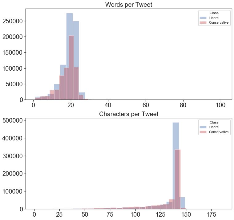
Get Character and Word Counts per Tweet

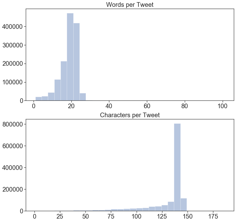
Who has longer tweets, Liberals or Conservatives? To judge we will make histograms of the distribution of “Tweet Length by Character” and “Tweet Length by Word.”

tweets_clean_df['words_per_tweet'] = [len(x.split(" ")) for x in tweets_clean_df['tweet'].tolist()]
tweets_clean_df['chars_per_tweet'] = [len(x) for x in tweets_clean_df['tweet'].tolist()]

tweets_clean_df[['words_per_tweet','chars_per_tweet']].sample(10)

	words_per_tweet	chars_per_tweet
748989	4	42
761081	13	98
581458	19	127
763005	20	146
674677	17	143
1172019	16	129
136311	16	137
432322	26	140
491182	20	140
550561	19	140

Combined Distribution of Tweet Lengths.

This distribution includes Conservative and Liberal Tweets.

It looks like Tweets are generally around 20 words or 140 Characters.

char_count = tweets_clean_df.chars_per_tweet.tolist()
word_count = tweets_clean_df.words_per_tweet.tolist()

f, (ax1,ax2) = plt.subplots(2,1,figsize=(12,12))

# set color theme
sns.set_color_codes("pastel")

# --------Top Plot-----------------
sns.distplot(word_count, kde=False,
             bins=30,
            ax=ax1).set_title("Words per Tweet",
                             fontsize=20)
ax1.tick_params(labelsize=20)

# ----------lower plot ------------
sns.distplot(char_count, kde=False,
             bins=30,
            ax=ax2).set_title("Characters per Tweet",
                             fontsize=20)
ax2.tick_params(labelsize=20)

Distribution of Tweet Lengths by Class

The trend of tweets being about 20 words or 140 characters seems to be shared by both Liberals and Conservatives.

No significant difference in the distribution of tweet length between Liberals and Conservatives is apparent.

Next steps

Now that we understand the data the next steps are to prepare the data for modeling and to build the model!!